Data Analysis

There are three main analyses in Biodiverse, moving window (spatial) analyses, cluster analyses and randomisations. These are described here, following a description of the spatial index which you would normally want to use to speed up any spatial conditions used in the analyses.

A fourth analysis type is the Region Grower which is a simple form of complementarity analysis, e.g. to find the set of groups that maximise the shared richness. It is actually implemented using the cluster analysis algorithm with the cluster metric set to maximise the index of choice. The interface is almost the same as for cluster analyses so it is not described here.

Building a Spatial Index

We will build a spatial index for our new BaseData object. A spatial index enables analyses using this BaseData to run faster (though beware that some user-defined spatial conditions will not work with a spatial index). Note that an index can be deleted/rebuilt at any time, and these changes affect only subsequent analyses, not those that preceded any change. If you are testing different index sizes using the same BaseData, delete previous analysis outputs to avoid reusing cached neighbour sets.

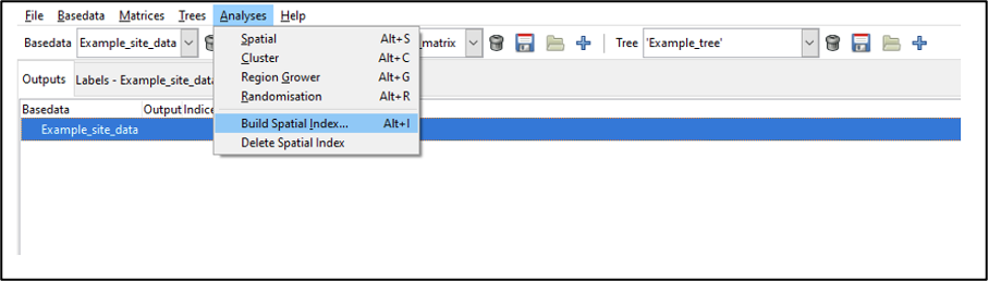
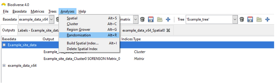
Select Build Spatial Index from the Analyses menu option:

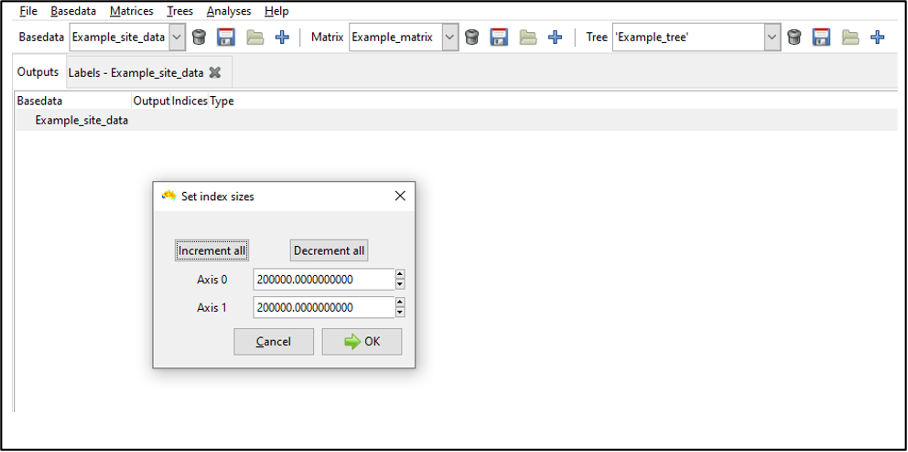
For most purposes, accept the index sizes suggested by the system (see here] for additional details on setting optimal index sizes). Note that index size refers to how finely Biodiverse divides spatial data into blocks for faster neighbour searching. Smaller blocks maximise precision but may involve more comparisons to identify the set of blocks to search (longer processing time). Larger blocks may compromise precision for faster processing time.

Click OK to build the spatial index. A pop-up dialog notifies you that the index has been built (OK).

Running a Spatial (Moving Window) Analysis

Introduction

The Spatial Analyses are a moving window analyses (because nearly all analyses in Biodiverse are spatial in some way) and are another method of identifying spatial patterns in your data. Depending upon the exact nature of your data, it is likely that the Groups comprising your BaseData constitute a geographic surface. Moving windows are used to systematically iterate across this space, with one or two neighbourhoods of the moving window being used to assess the labels/values aggregated in the Groups. The window might also consist only of the processing group, with no neighbours (each group is analysed separately).

To run a moving window analysis, you will need to have imported or loaded a BaseData object and ideally built a spatial index for this BaseData. These instructions assume you have either imported the sample data above, or you can open the example BaseData object ’example_data.bds’in the Biodiverse data folder.

Select a Basedata object by clicking on it and open the menu option Analyses -> Spatial and the spatial tab appears:

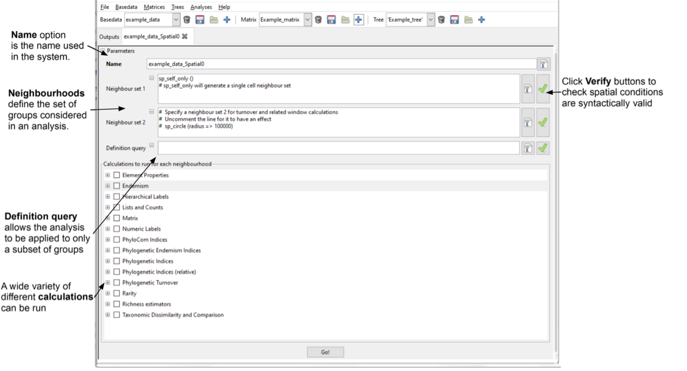
The Spatial tab has two main sections where you can set options. The upper section (Parameters) determines the parameters used in defining the two neighbour sets used in the spatial analysis (the second is optional) as well as the definition query. The lower (Calculations to run for each neighbourhood) determines the subsequent calculations that will be run for the set of neighbours related to each group. You can select any number of calculations to perform.

Setting the Spatial Analysis Options

The Name option is the name used in the system. You can accept the default, or enter a new name (you cannot have duplicate names within the same BaseData object).

The Neighbour set 1 and Neighbour set 2 text boxes allow you to define the neighbour sets used for the calculations (see the Spatial Conditions documentation for further details). The size and shape of the neighbourhoods define the set of groups considered in an analysis. It is up to you to decide what sort of neighbourhoods and how many to use for your analysis. The system provides considerable flexibility in this regard: both neighbour sets may be arbitrarily defined independently of each other, and you are not obliged to specify a second neighbourhood.

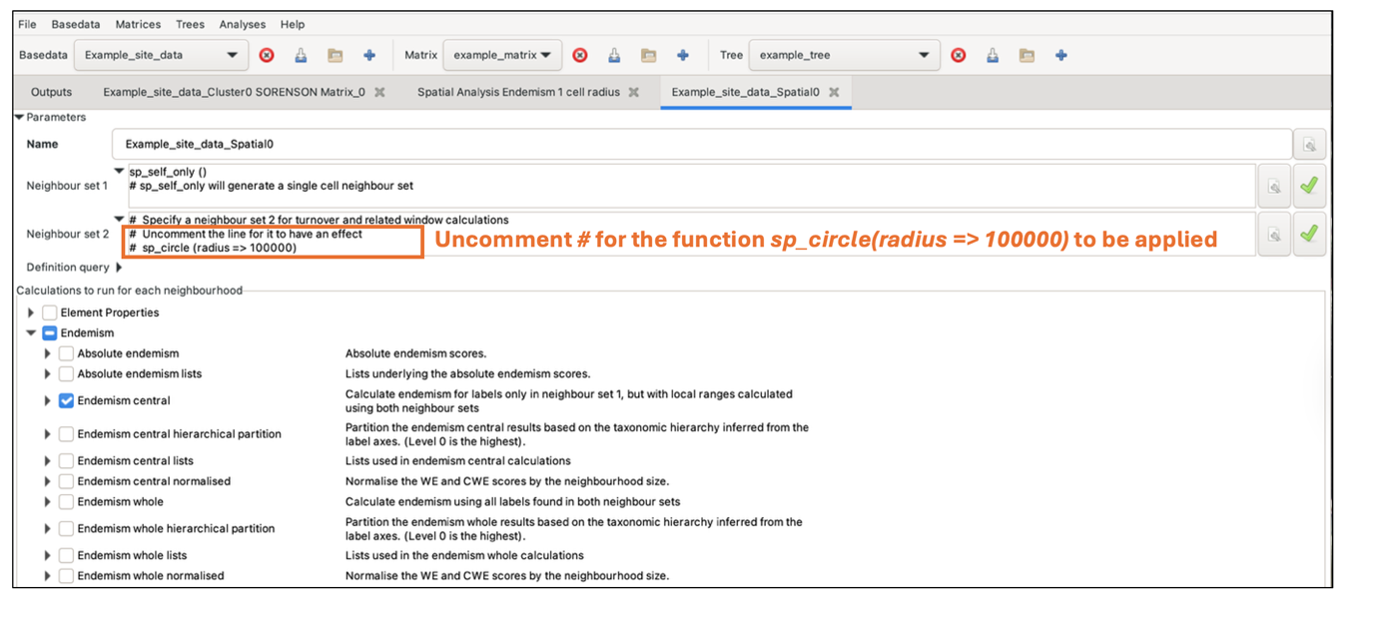
The default condition in the Neighbour set 1 text box is sp_self_only(). This restricts the neighbourhood to one cell/group (the processing group, which is the group being processed at an iteration). The default condition in the Neighbour set 2 text box sp_circle (radius =\> 100000) defines a circular neighbourhood of 100000 units centred on the processing group. The units are whatever the original data used, and for the example data, this is a 100 km or one cell radius. Make sure to uncomment the # for the function to be applied.

These default conditions are appropriate for our sample data, but we will modify the second condition. Change the circle radius from 100000 to 200000.

See Spatial Conditions for more detail on defining the neighbourhood sets (e.g. for the range of functions that you can use to specify neighbourhoods).

Note that the use of neighbourhoods varies according to the type of calculation selected for analysis (see Selecting Indices below). Some calculations aggregate the neighbourhoods into a single set (e.g. endemism_whole), others compare the labels in the first neighbour set with those in the second (e.g. Jaccard and other dissimilarity indices), while others use the first set to define the list of labels to use but then consider distributions across both neighbour sets (e.g. endemism_central). Some will not be run unless two neighbour sets are defined, primarily the turnover calculations.

The Definition query text box allows the analysis to be applied to only a subset of groups, as described in the setting cluster analysis parameterssection above (those which satisfy the criteria in the definition query, but note that all groups are still considered as possible neighbours).Leave this blank for this session. For details of setting a definition query, see Definition Queries.

The Verify buttons let you know if the spatial conditions entered are syntactically valid.

Selecting indices to calculate

In the calculation section, use the check boxes to select which indices you want to calculate. For the sample session, click the arrow buttons next to the Endemism, Lists and Counts and Taxonomic Dissimilarity and Comparison to display their subsets. Select Endemism central (Endemism), Redundancy and Richness (Lists and Counts) and Sorenson (Taxonomic Dissimilarity and Comparison). Note, if the parent category is selected (e.g. Endemism), all subset indices within that set will be calculated.

Details about the full range of indices are available from the Indices documentation.

Click on the Go! button. The system will then run the selected spatial analyses.

Viewing the Spatial Analysis Results

Once the analysis is complete, the system asks you whether you want to display the results. Click Yes and you will be shown a map of the moving window analysis results. Pull the pane down to view the options you used, for example to change them and re-run the analysis.

At this point, it may be useful to use the Overlays function (explained here) to analyse results in their geographic context. Note that currently, adding an overlay can slow processing time when wanting to pan, select or hover over groups and nodes.

Running analysis with local neighbours

In the above moving window spatial analysis, the output visualisations only provided a single cell output of iterations within the map (black dot within the group cell).

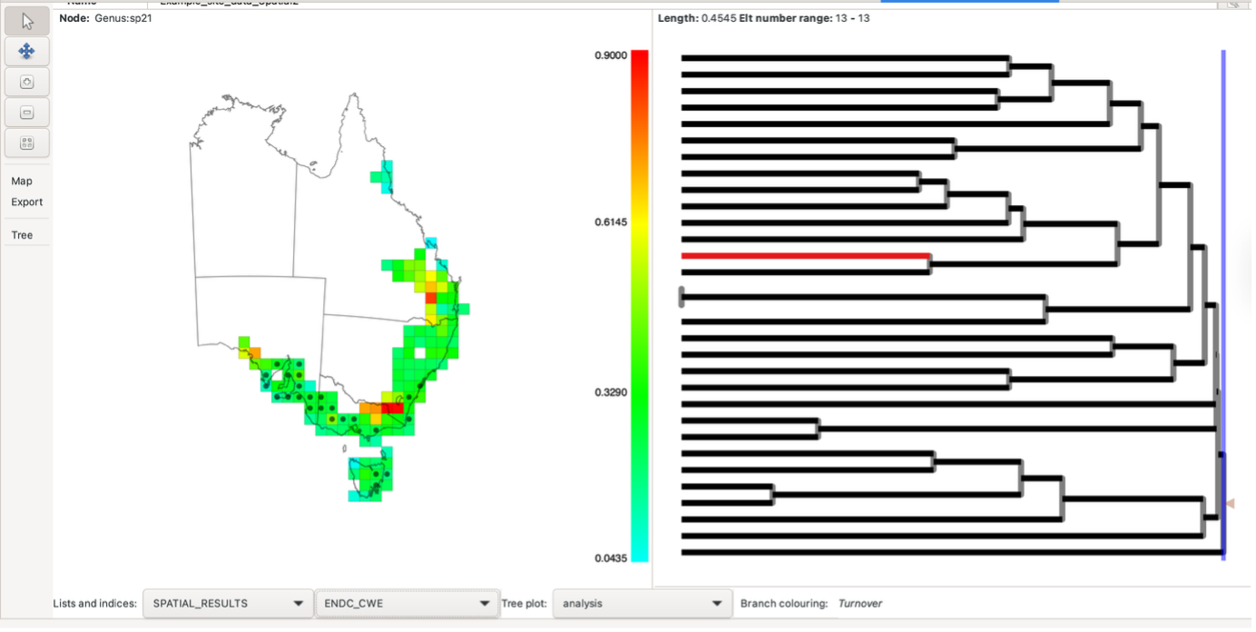
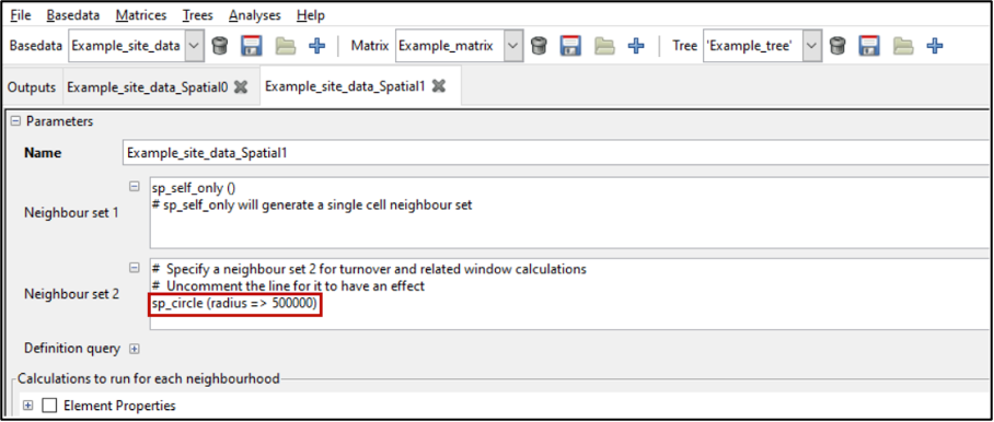
However, altering the second neighbour entry to sp_circle (radius => 500000) when setting the initial analysis parameters (noted above), can identify aggregated relationships of these cells with their “neighbours”.

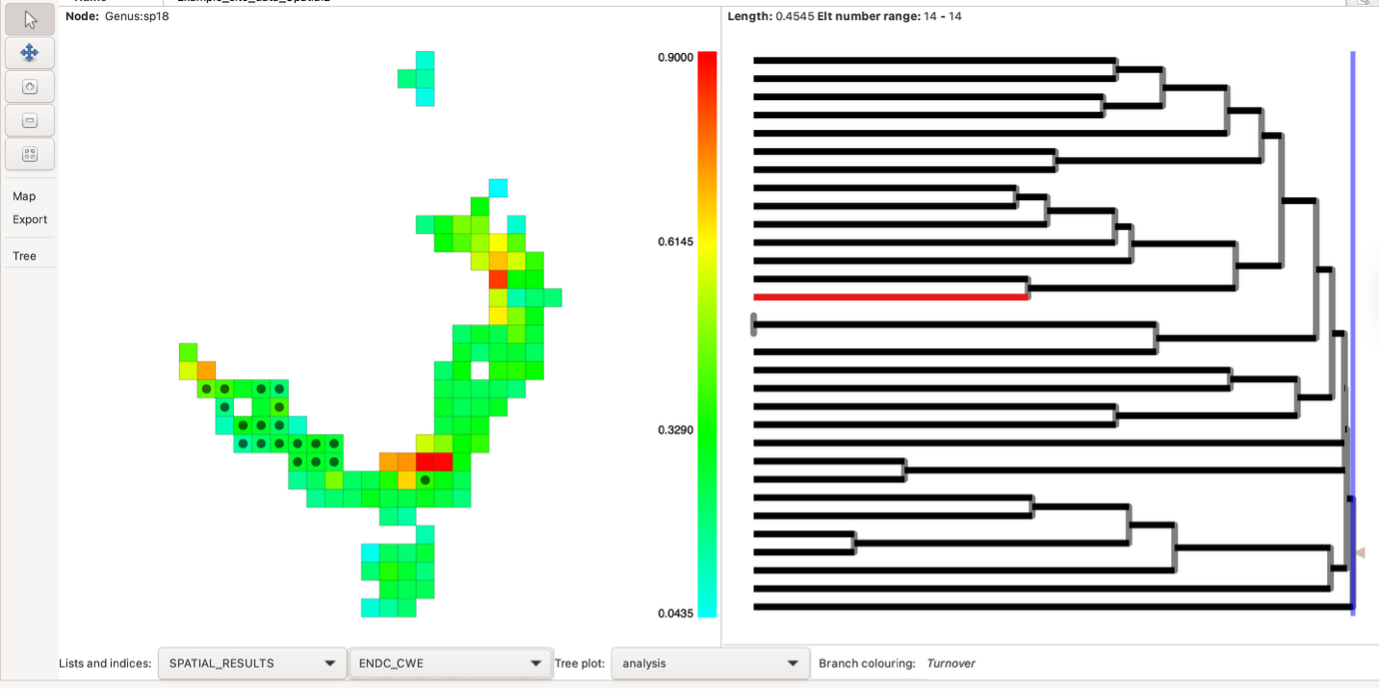
The result is a display like this:

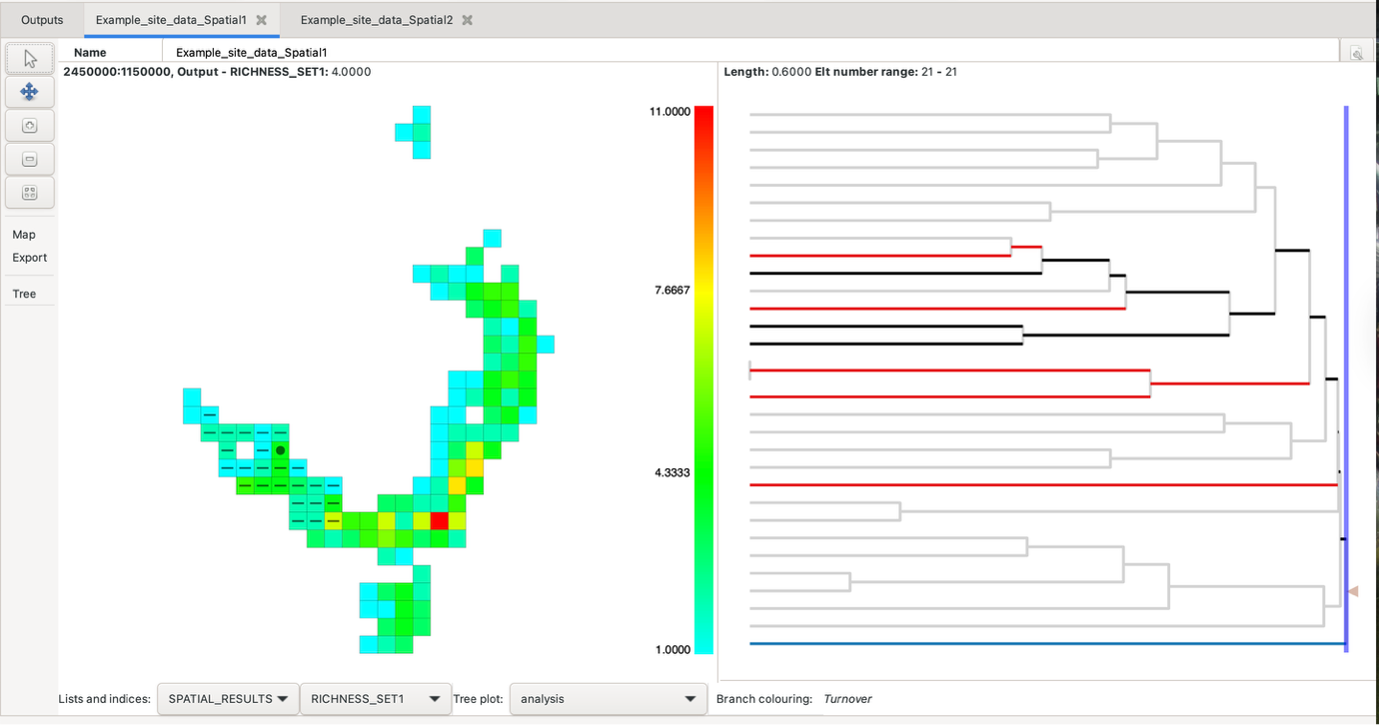
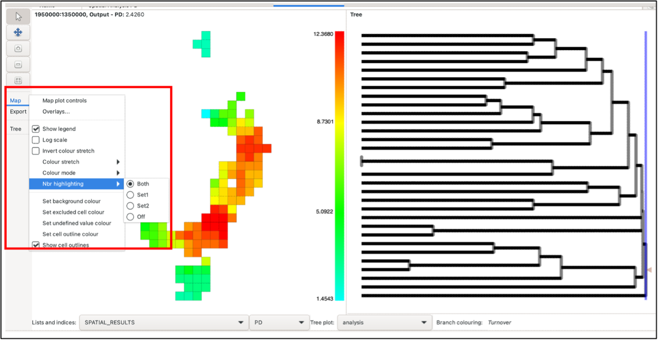
Hovering over a group will highlight the groups used in the calculations, a solid circle for those in the first neighbourhood and a dash for those in the second neighbourhood. Right-click on a group to keep the highlighting at that group until the mouse is left-clicked on any group. You can control whether these are displayed or just display one set by using the Nbr highlighting option under the Map list in the left-hand toolbar.

Holding the control key while clicking on a group, or clicking on a group with the middle mouse button, produces a pop-up list with all the results in it. It also includes lists of the elements (groups) in each neighbour set (Elements set1, set2 and all) and of the labels in these neighbour sets (Labels set1, set2 and all). The “All” list is the union of neighbour sets 1 and 2.

The tree branches are coloured according to whether they are found only in the first neighbour set (blue), the second neighbour set (red), both (black) or neither (grey). The screenshot above displays this. Also see the blog post. Some indices can also be plotted on the tree.

Running a Cluster Analysis

Once you have imported or opened a BaseData object, you can run cluster analyses to identify clusters in this data.

Biodiverse supports agglomerative clustering of the groups based on their labels, or some function of their labels such as the values of a linked matrix or tree.

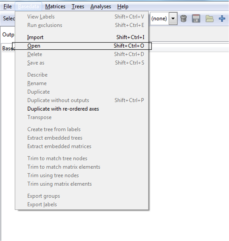
We will run a cluster analysis on the BaseData imported earlier ‘Example_new_basedata’ (see Importing data). If My_new_basedata is not loaded, but you have saved it, open this file now by clicking on ‘Open’ from the Basedata menu and navigating to the location of your bds file.

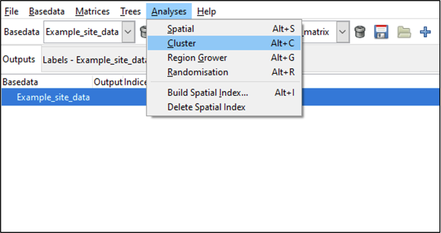
To run a cluster analysis on the currently selected BaseData object, select Cluster from the Analyses menu:

The cluster analysis tab opens. It has three main sections where you can set options:

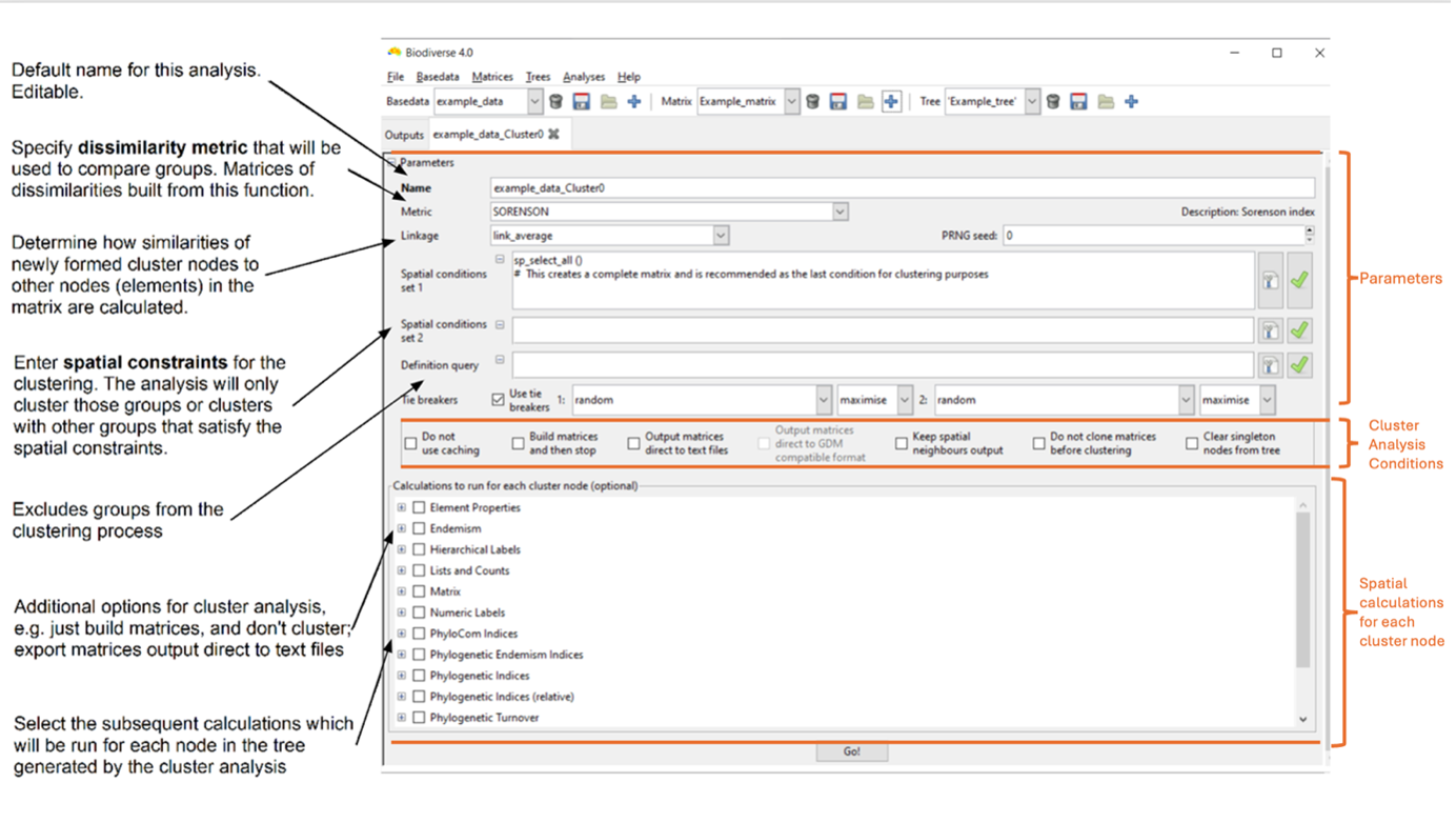
• The upper section (Parameters) determines the parameters used in the clustering to generate a tree. This includes options to control the cluster tie-breaker algorithm.
  
• There are check-boxes in the middle section that can be toggled to alter how the cluster analysis runs, e.g. by controlling aspects like process performance (e.g. memory usage), the automatic export of results, etc.
  
• The lower (Spatial calculations to run for each cluster node) determines what subsequent calculations will be run for each node in this tree, using the groups it contains to define the spatial sample. This allows you to, for example, calculate the phylogenetic diversity of the regions defined by each cluster node.

Setting cluster analysis parameters

For this guide, accept the default name for cluster analyses (see the diagram above) and the default metric, ‘SORENSON’ (the set of indices available for clustering is shown in the “Grouping metric?” column in the Indices list), which includes tables summarising all supported metrics and indices by Biodiverse. If the column is blank, the metric cannot be used. Also accept the default linkage, ‘link_average’, which calculates the dissimilarity of each new group with all others as the average of the groups merged to create it, weighted by the number of terminal nodes each contains. This means a merge between node A with 10 terminal nodes and node B with 1 terminal node will not be biased towards node B’s labels. See the Cluster parameters section of the Sample Session for details of other available linkage functions.

The spatial conditions can be used to control which Groups are considered candidates to be clustered together. The default condition in the ‘Spatial conditions set 1’ text box provided by the system is sp_select_all() This condition selects every group and is an appropriate condition to use for unconstrained clustering. If you wish to use a different spatial condition, for example, to first cluster within geographic regions, then refer to the Spatial Conditions documentation for further details).

The definition query serves a similar purpose, except that it can be used as a filter to restrict the clustering to only a subset of groups. For example, you might have a data set for Europe but only want to cluster cells in regions above a specified elevation value. The Spatial Analysis section in this document provides additional details about spatial conditions and definition queries.

Tie-breakers deal with groups that have the same similarity score as the processing group. Tie-breakers create rules to determine which group should be merged first, using a user-selected index. If your project has a specific conservation focus, tie-breakers can bias clustering toward areas with higher richness, endemism, or other priorities.

Tie-breakers are mainly useful when the matrix has similar values, e.g. there are many groups with the same labels. The tie breaker is used to decide which groups should be merged next in the clustering process.

For example, two clusters have the same similarity score, but Cluster A has high endemism and Cluster B has low endemism. If the primary tie-breaker is selected as ENDW_WE (Endemism Whole) to maximise, Biodiverse will merge with Cluster A because it has higher endemism. A secondary tie-breaker can be chosen (e.g. random), meaning if the primary tie-breaker still results in a tie,Biodiverse picks randomly.

Check the option or calculations boxes as appropriate. If you’re curious as to what they do, hover over them with the mouse pointer to view a tooltip.

Click on the Go! button (keyboard shortcut Control-G). The system will first build the dissimilarity matrix (or matrices if you have several spatial conditions), then run the clustering using these matrices, and then any spatial calculations you have selected for each node. It will then prompt you to display results.

Viewing the cluster results

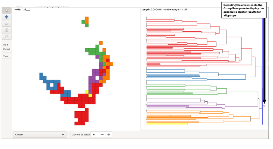
There are three sub-panes within the display pane. On the left is the group grid, on the upper right is the tree representing the clustering, and on the lower right is the scree plot for the tree.

As with the visualisation of BaseData/Matrix Tree objects described earlier, the system is linked, and interactions in the group grid or tree of the cluster display are generally reflected in the other. Hovering the mouse over a node in the tree highlights the groups (in the group grid) that are contained in that node with a black dot. Likewise, hovering the mouse over a group in the group grid will highlight the path (set of nodes/clusters) in the tree to which that group belongs.

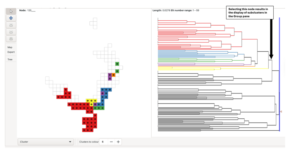
To view clustering analysis results for all BaseData, left-click the arrow at the right-most side of the tree pane. This selects the root branch, which may have a zero length. The number of clusters displayed can be adjusted using the “Colours to clusters” feature. Note there is a maximum of 13.

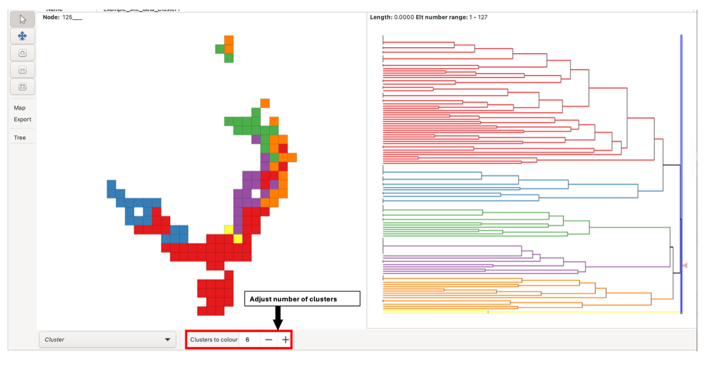
Alternatively, the blue sliding bar in the tree pane can be dragged across the tree to colour/cluster the nodes and groups at that level (e.g., a bar dragged over two nodes generates two clusters). The bar displays the number of nodes it is crossing when the mouse is focused on it. If the slider bar crosses more than 13 nodes, all nodes will be uniformly coloured red instead, and groups in the group grid will not be coloured.

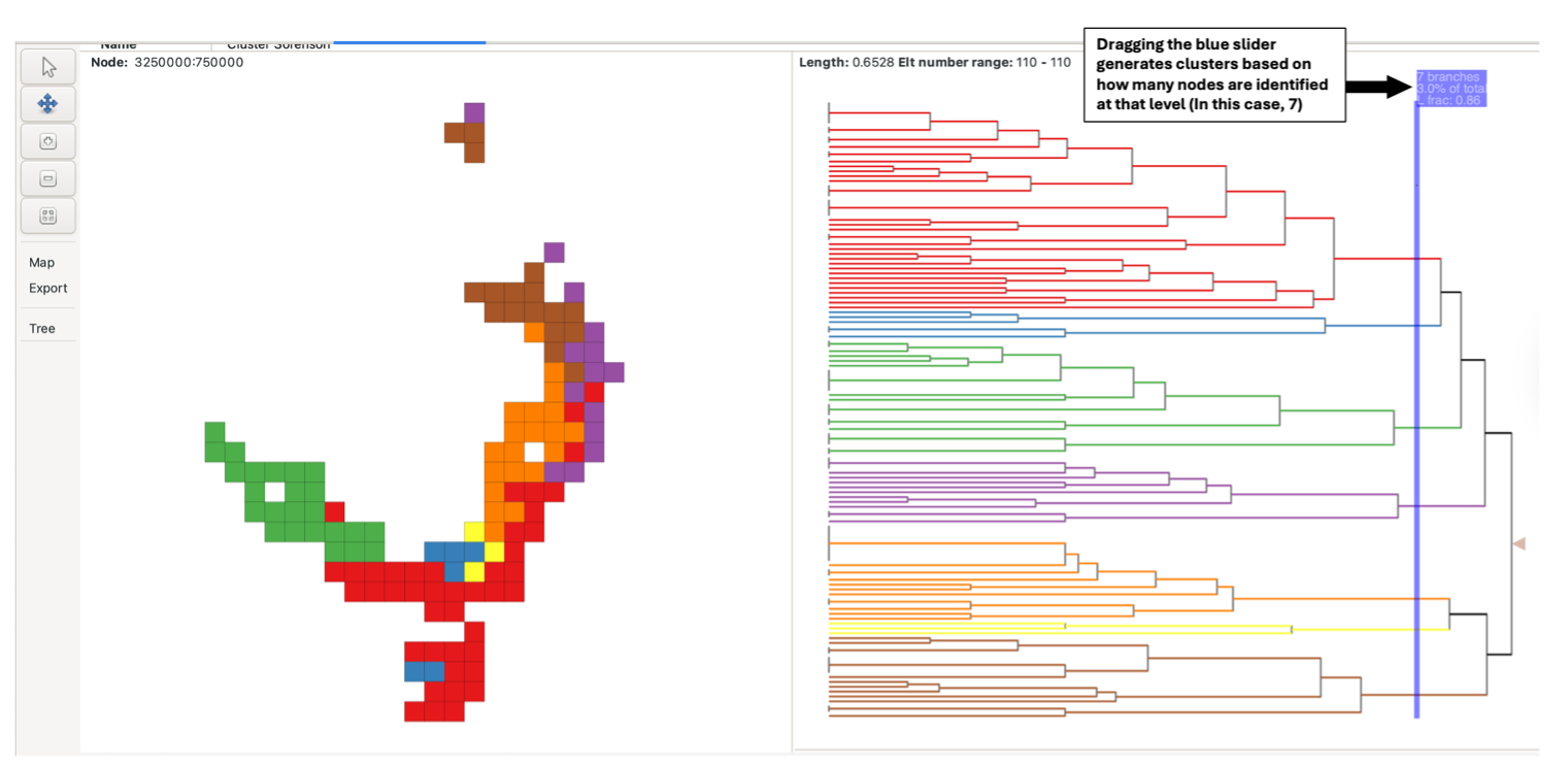
Left-click on a tree node to colour a set of subclusters (descendant nodes in the tree). These clusters are split into coloured groupings based on the “Clusters to colour” parameter at the bottom of the pane. Note that some leaf nodes in the tree may have a length of zero (indicated by vertical bars at the leftmost side of the tree, longer vertical bars indicating more zero-length leaf nodes). Thus, if any such nodes occur under (to the left of) the node you have selected, their colouring will not be apparent if you are using “Plot by Length” mode. These nodes, along with their colouring (if selected), can be made apparent by switching to “Plot by Depth” mode under the tree options button under the Display menu at the left.

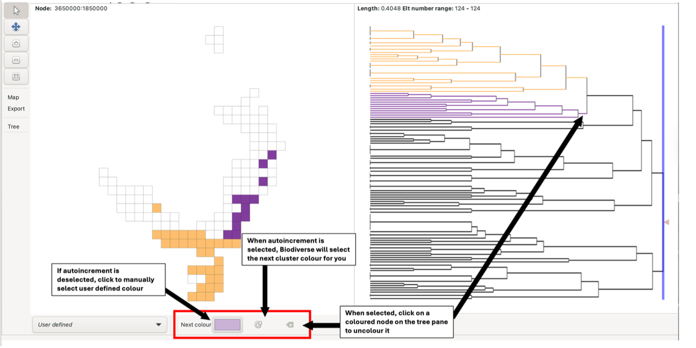
It is also possible to [assign your own colours to the clusters](https://biodiverse-analysis-software.blogspot.com/2016/09/new-selection-tool-in-cluster-analysis.html and to generate a geotiff (raster) to reproduce the coloured cells in other systems.

This function is useful if you wish to visually align the Biodiverse cluster results with existing datasets (e.g. Bioregions)

To do this, select user-defined in the selection list on the bottom toolbar. Select the preferred colour and then fill the group grid by selecting your user-defined cluster node on the tree pane. Selecting the autoincrement button will allow the system to select the next colour for you; deselecting this will keep the cluster colour the same until it is changed manually by the user. The deselect button allows you to uncolour clusters by selecting them on the tree pane.

The cluster analysis generates a dissimilarity matrix, which can be selected and viewed in the Outputs tab. In the example case, the index used is Sorenson, but a matrix can be created for different indices.

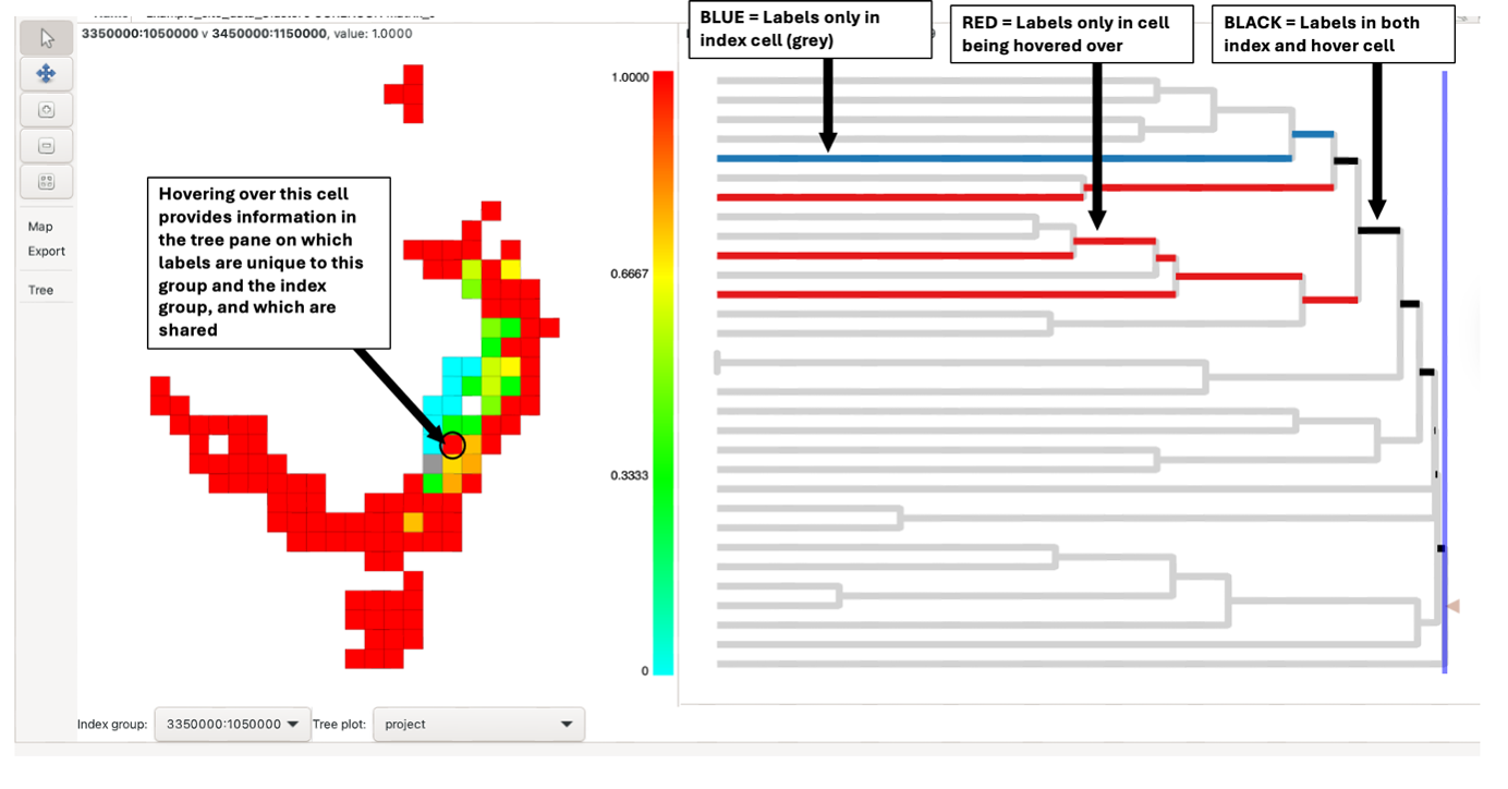
The results consist of a map and a tree pane. The map illustrates the degree of similarity or difference between each group and its cluster neighbours. By hovering over or right-clicking a group (index group), its dissimilarity value is displayed at the top of the map pane.

Right-clicking a group selects it as the “index group”, and the cell will be filled in grey. When an index group is selected, the map colourings will change to display the dissimilarity of all groups relative to the selected group. The map colouring indicates the dissimilarity value from 0 (low dissimilarity – sites are similar) (blue) to 1 (high dissimilarity – sites are different) (red). Other groups can be hovered over whilst the index group remains selected.

When an index group is selected, the label (node IDs) contained within the group are highlighted in the tree pane in black.

Note that hovering over different groups whilst the index group is selected will highlight additional branches. Blue branches are found only in the index cell; red branches are found only in the cell being hovered over. The branches in black are found in both neighbouring cells. Branches not found in the two cells are in grey (reduces visual impact without hiding it). See this blog post for further information about how Biodiverse visualises phylodiversity.

Running a Randomisation Analysis

Introduction

Randomisations in Biodiverse are used to assess the statistical significance of a set of analysis results given some randomisation scheme, such as shuffling the species around the map (labels across groups in Biodiverse terms), subject to constraints such as each cell (group) must maintain the same number of species. Randomisations are key to interpreting where results differ from what would be expected, and are integral to protocols such as the Categorical Analysis of Paleo and Neo Endemism (CANAPE). The output can provide rank-relative scores from which significance can be derived,as well as z-scores.

The default randomisation algorithm in Biodiverse is called rand_structured.

The rand_structured algorithm is so called because it maintains the structure of the original data, specifically the spatial distribution of the richness patterns, while randomly allocating taxa (labels) to groups (cells). By default, the richness patterns are matched exactly, but users also have the option to allow tolerances such as an additional number of labels per group (e.g. five extra), or some multiple of the observed (e.g. 1.5 times as many). The rand_structured randomisation uses a filling algorithm, followed by a swapping algorithm to reach its richness targets. There is a series of blog posts describing the randomisation algorithms and visualisations.

The basic process of the randomisation is this. For each iteration of the randomisation analysis, Biodiverse will:

1. Create a new BaseData object with a random allocation of labels to groups, according to the selected algorithm
   
2. For each analysis in the BaseData:
   1. Regenerate a version using the randomised basedata
      
   2. Compare the values of the analyses from the original and randomised BaseData and track if they are higher or lower, on a group by group basis
      
   3. Track basic statistics of the distribution to allow the calculation of the mean and standard deviation, and thus z-scores.

Randomisations can be run by selecting the Analyses>Randomisation menu option:

Cluster and Region Grower trees are not rebuilt by default, partly for speed, partly because it is not normally needed. If you do want to do so then select the “build randomised tree outputs” checkbox. Note that any calculations per node are compared against the randomly generated basedata, though.

The PRNG seed option allows the user to run reproducible sequences of random values between randomisations. If you set the same seed, you will get the same randomisation results every time you run it (with the same settings). If you leave it blank or change it, the randomisation will produce a different result.

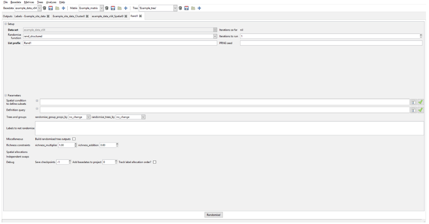
Once the relevant parameters are specified, press “Randomise!”.

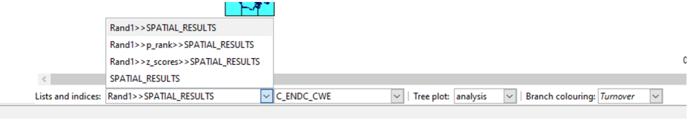
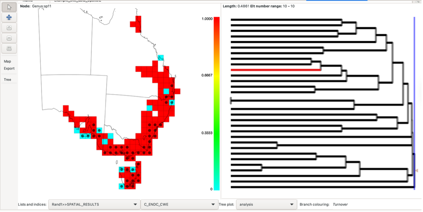
Note that the randomisation analysis tab does not show maps or any other displays once the specified number of iterations have completed. The results are added as lists to any existing analysis objects and can be displayed by selecting from the “List and Indices” option on the relevant plots. You might need to close any open plots and re-open them to see the new lists. See the main help system.

A description of what the list and index names mean is also in the main help system. (Consider for example the Rand1>>SPATIAL_RESULTS list and C_END_CWE index below).

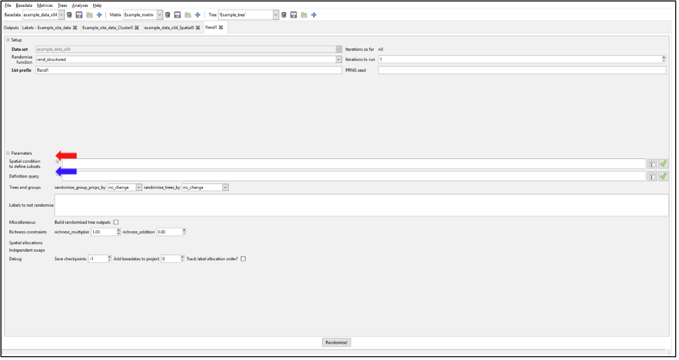
Spatially Structured Randomisations

In the standard implementation of randomisation, labels are assigned randomly to any group across the entire dataset. This approach works well for many studies and is very effective. However, as analyses scale up to larger extents, the total pool of labels begins to span many different environments. The randomisations might assign a polar taxon to the tropics, and a desert taxon to a rainforest. While this does not make the randomisation invalid, it may be less strict and less realistic than it could be.

This can be readily fixed in Biodiverse by specifying a spatial condition to define subsets. Or, if you only want to randomise a subset of your data while holding the rest as-observed, you can use a definition query. You can specify spatial conditions using the same syntax as for the Spatial and Cluster analyses. The analytical decisions are yours but generally, it is better to use a condition that generates non-overlapping regions. Each group is allocated to only one subset, so in such overlapping cases it is the first one that contains a group “wins” that group.

Additionally, you can set some labels as constant, giving greater choice depending on the analysis aims. This may be useful for endemism studies, where you want analysis results to reflect real-life ecological restraints on distributions.

To read more on spatially structured randomisations see this blog post.