Importing Data
Note: If all your files are in the same location then you can set the working directory under the File menu to save time finding them. You can also bookmark folders in the file selector to get back to them more easily. Right click on a folder to see the option.
Data structures
Before importing data it is important to understand the sorts of data supported by Biodiverse. There are four main types, each of which can be stored in native Biodiverse format.
Projects – (file extension .bps) are a composite structure and may consist of a set of any number of BaseData, Tree and Matrix objects and any associated analysis results. These are only used by the GUI.
BaseData – (file extension .bds) is the primary storage object used in Biodiverse. BaseData stores your spatial data (e.g. different species and their XY locations), a set of analysis parameters, and any associated outputs from cluster, moving window and/or randomisation analyses.
Trees – (file extension .bts) these are hierarchical tree structures, e.g. phylogenies, taxonomies or word roots, which are imported from nexus and similar formats. These are used for analyses involving tree structures, e.g. phylogenetic diversity, linked by the matching labels in a BaseData.
Matrices – (file extension .bms) these are matrices of numeric values representing some relationship between pairs of labels or groups. These are used for analyses involving matrix structures linked by the matching labels in a BaseData. They are also used as part of cluster analyses, in which case they relate to pairs of groups in a BaseData object.
Opening data
To open pre-existing data (i.e. a Project, BaseData, Matrix or Tree saved to disk), select Open under the desired menu option and then navigate to the relevant file to load it:
 Or click
  on the relevant menu bar.
Select the file you want to load, and click OK.
Importing data
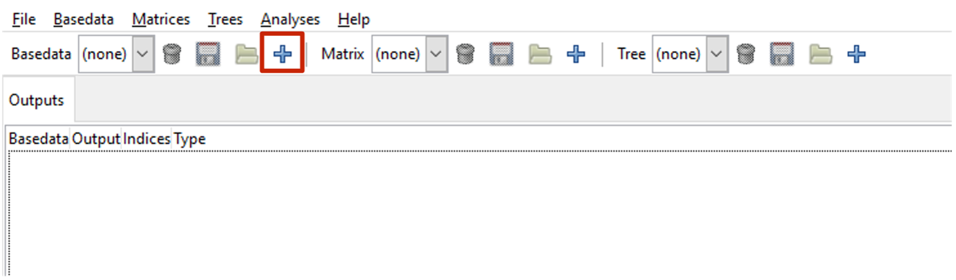
BaseData, Matrix, and Tree object data can be imported from ‘raw’ data files (e.g. Tabular text, rasters, shapefiles, spreadsheets or CSV text files in the case of BaseData and Matrix objects) by clicking on their respective import buttons  on the main toolbar, or via the ‘Import’ command in their respective menus.
For BaseData objects, either a new object can be created, or an existing object can be added to. When adding data it is up to the user to ensure the new data are in the same coordinate system (i.e. Biodiverse does not check if you add data in UTM coordinates to a BaseData object using decimal degrees).
BaseData
The default import file type for BaseData is delimited text (e.g. CSV files) but you can also import from shapefiles, spreedsheets and geospatial rasters.
These instructions describe the process where an input text file is in list format and contains one record per observation, with separate columns for one or more labels (e.g. names such as genus and species) and groups (e.g. x and y coordinates of a data point). However you can also import data from raster, shapefile and spreadsheet formats. All formats except raster can also represent a matrix of data such as for a sites by species matrix (see Importing Data in Matrix Format).
See the Example_site_data.csv file in the data folder for an example of the file format. The columns of data can be separated by commas, spaces, tabs, semicolons or some other user defined character. There is no restriction on column names or how many columns there are in the file but it is up to the user to know what they represent. You can allow the system to determine the separator type or select from a range of options.
| num | genus | species | x | y |
|---|---|---|---|---|
| 1 | Genus | sp1 | 8 | 8 |
| 2 | Genus | sp1 | 6 | 2 |
| 3 | Genus | sp1 | 8 | 9 |
| 4 | Genus | sp2 | 5 | 4 |
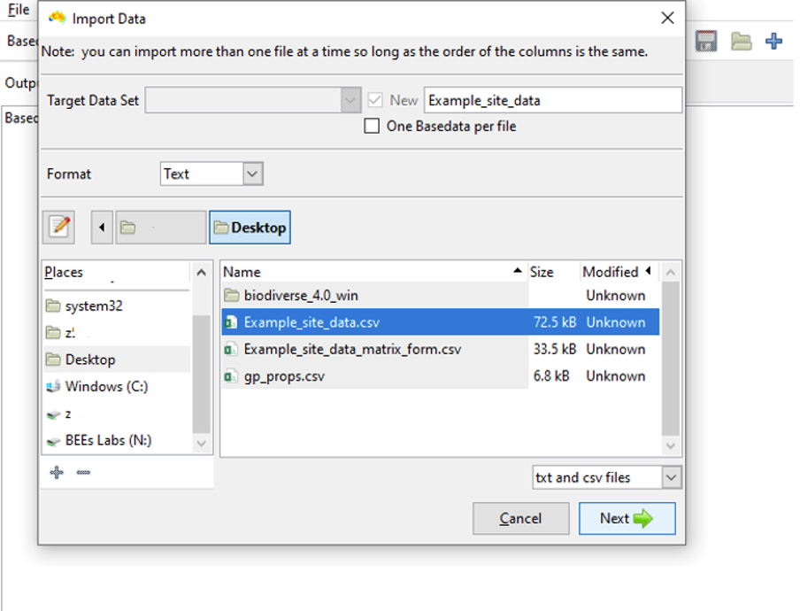
Select the import button on the BaseData toolbar (or use menu Basedata>Import) to open the Import Data dialogue window, from where you can select the input data file.
The text box at the top right of the Import Data window allows you to name the output BaseData object that will be produced. Once you are finished, click Next.
You will then see the Import Options window with various options you can set for the import:
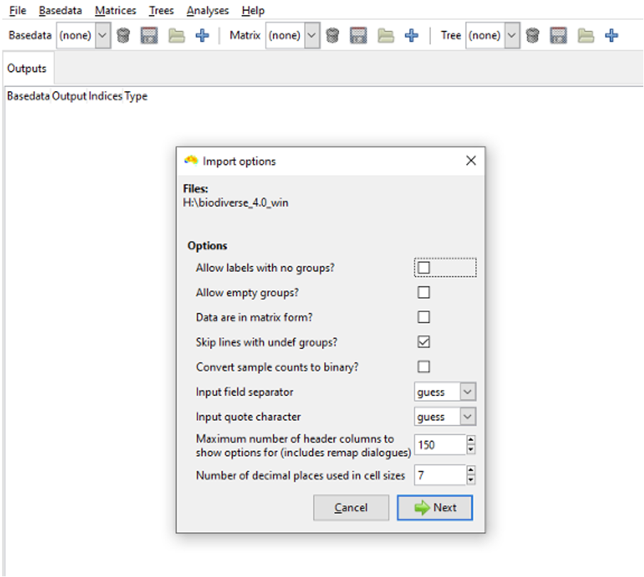
More details of the import options are in the Import Options page, but leave all of them unchecked for this tutorial, except ‘Skip lines with undef groups’. Checking this option allows you to ignore records where a group field is either undefined or non-numeric. Such records can occur where you do not know the coordinates for a sample, if you choose the wrong column to use for the groups, or if you have a series of lines with no data at the end of a file.
If you are not importing the Example_site_data.csv file, bear in mind you might need to check some of the other import options. A useful option is ‘Allow empty groups’ which lets you have groups that are considered for analysis, but that have no labels themselves. This is useful when you wish to have moving window analyses extend beyond the sampled data to give a smoother result.
Click Next.
The Choose columns dialog box appears and allows you to select various options for each column in your input text file.
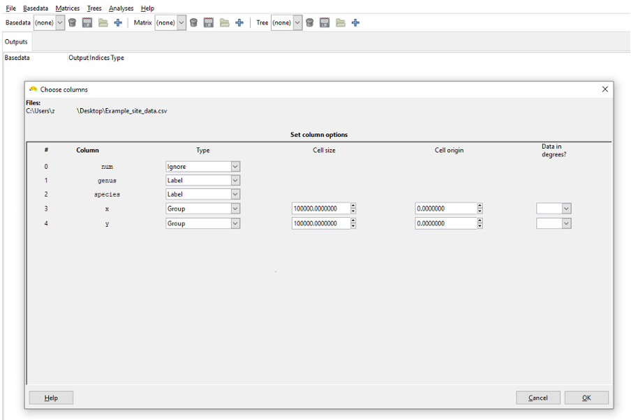
You must set a Type value for at least one Group and one Label column, but more than one of each may be chosen.
All columns in your file that are irrelevant to the analysis should be set to Ignore, as is done for the num column in this case.
Select Label as the Type for the genus and species columns. This represents genus and species values for each record as one combined label, i.e. ‘Genus species’.
Select Group as the Type for the X and Y columns.
When a Group column has been set you will be given the option to select its cell size (in the same units as the group data is stored) and its origin. If you are not importing the Example_site_data.csv file, make sure these dimensions and units are appropriate to your data. You can specify if the group data are degrees using the Data in degrees? comboboxes. This allows you to import data in degrees minutes seconds (e.g. 22° 15’ 10’’ S) and decimal degrees formats, as well as enabling some validation that the coordinate values are in the correct range for such units.
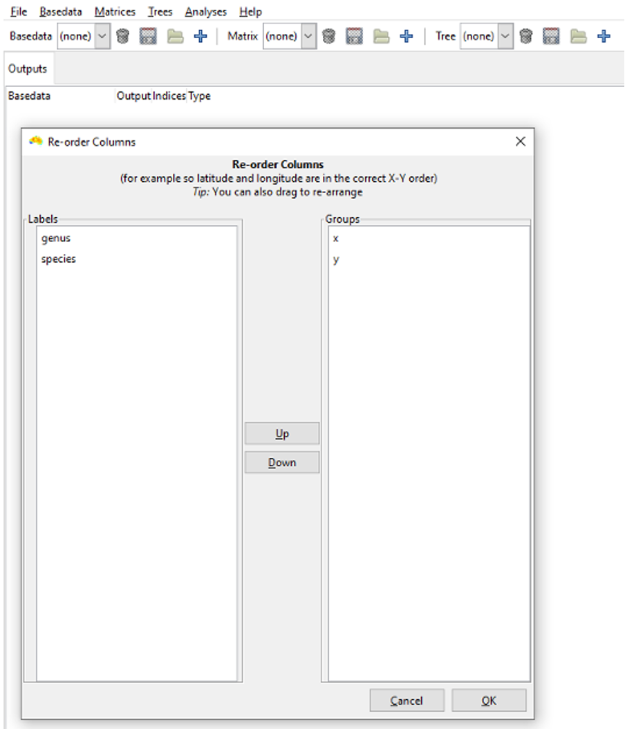
The Re-order Columns dialog box is the next window to appear. This allows you to order your labels and groups. For example, placing “y” above “x” makes the y column data the first dimension of a group’s coordinates and x the second (useful if latitude precedes longitude in the column order of your input file). If you forget this step then the axis order can be changed later on using the Duplicate with re-ordered axes tool under the BaseData menu.
Since the columns in Example_site_data.csv are already in the correct order, we will accept the current column ordering. Click OK.
Biodiverse now imports the data from the Example_site_data.csv input file and creates a new BaseData object. Once the import process is complete, the name of the new BaseData object (‘My_new_basedata’ in this case) appears in the top-left of the Biodiverse main window.
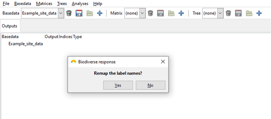
Remap
The option to remap (change) label names will appear after the re-order option.
The remap process can generate possible matches between spatial data and any tree, matrices, group properties and label properties automatically. Remapping is helpful when the user is working across multiple data sets and wishes to standardise components such as element names or spatial units. For example, where a set of labels needs to be altered in a tree to match the BaseData object labels (vice versa).
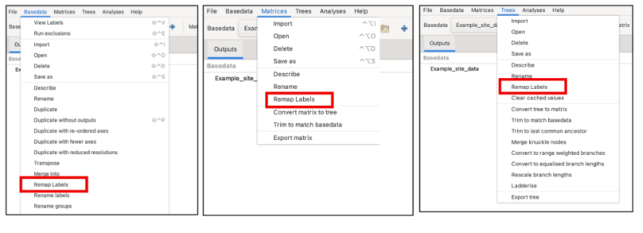
Whilst the user is prompted to remap when importing data, remapping can be performed during or after import. To remap after import, locate “remap label” under the BaseData, Tree and Matrix menus.
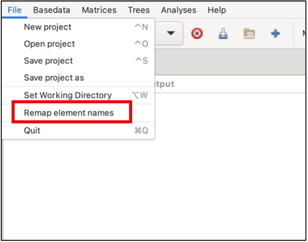
The centralised interface for automatic remaps can be accessed under the file menu, as below. There are panes listing exact matches, non-matches (i.e differences were too great), punctuation matches and possible typos. Users can choose to ignore any of these sets, and also select subsets within the sets if, for example, there are false matches. See the blog for further remap information and examples.
Since we are just importing example base data we will not remap so choose “no”.
Having imported data into a BaseData object, you are now ready to run cluster, moving window and randomisation analyses, or you can visualise this data (see Visualising Data) or calculate a spatial index (see Building a Spatial Index) which helps run faster analyses when using this BaseData. Alternatively, you can now import additional data files (see importing Matrices and Trees below).
However, prior to doing anything else, it is a good idea to Save your newly imported data. Use the File > Save menu option to save the whole project. To save just the BaseData select the My_new_basedata object, and save it as a BaseData object, either via the Basedata menu (Basedata > Save as) or the  icon on the Basedata toolbar.
Matrices
Matrix data can be imported at any time, although it can only be viewed with an existing (and selected) BaseData object. Currently only delimited text files can be imported (e.g. csv or txt files).
These matrices are not site by species matrices. These are matrices of numeric values representing some relationship between pairs of labels or groups, for example numbers of base pairs shared between pairs of labels. Site by species data are imported using the basedata import process.
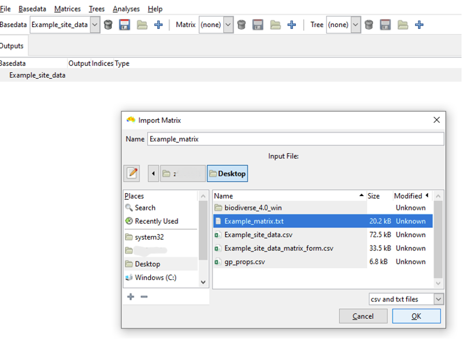
Select the import button on the Matrix toolbar to open the Import Matrix dialogue window, from where you can select the input data file. Select Example_matrix.txt, give the new Matrix a name if you like, and click OK.
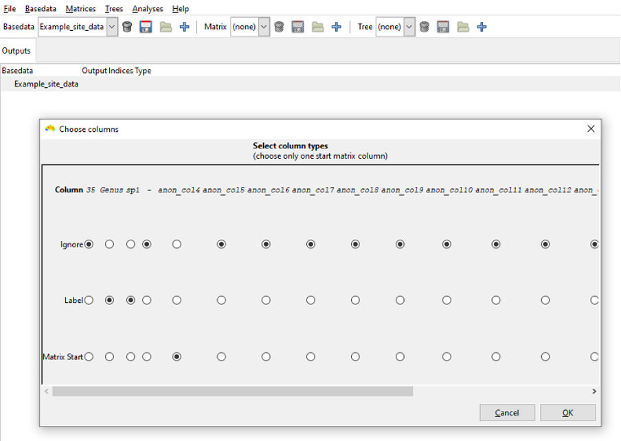
After deciding if your matrix input file format is normal or sparse, you must now decide how the columns in the matrix file should be read. You must select at least one label column, and only one “Matrix start” column. Any other columns in the file should be set to “Ignore”.
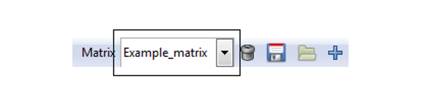
Click Ok, then select No when prompted to Remap element names and set include/exclude? The matrix is imported and appears in the drop-down menu in the matrix toolbar at the top of the screen.
The matrix can only be visualised once a BaseData object has been imported and visualised as well. (it will only produce a useful display if the matrix and BaseData share at least some labels).
Note that you can either save the matrix as a Matrix .bms object (‘Matrices > Save as’ from the menu), or it can be saved as part of a Project see Saving a Project at the end of this guide.
Trees
There are two options for creating Trees in Biodiverse:
Import a Tree into a project at any time
Derive a Tree at any time if you already have a BaseData and/or matrix object selected.
In both cases, a Tree can only be visualised with an existing BaseData object. A Tree is most useful if it shares some labels with the BaseData being displayed.
Importing a Tree A Tree can be imported from nexus (*.nex or *.tre), newick, “R json” or tabular formats. Once a tree is imported, it will be added to the project.
To import a Tree, select the import button on the Tree toolbar. A window will appear asking if your tree data are in a tabular format. After selecting YES or NO, you can select your file:
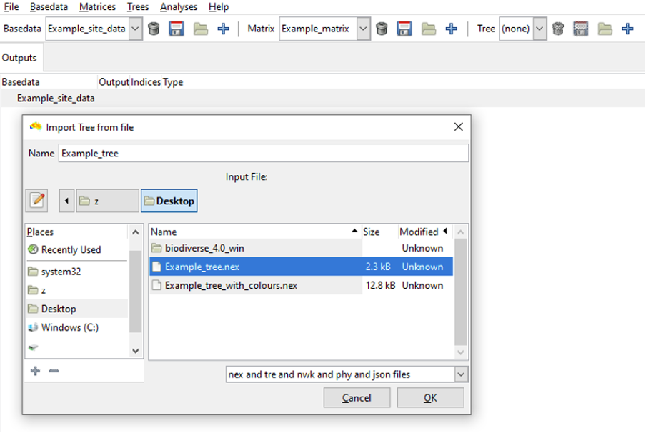
Select your file and click OK. You will then have the option of choosing a label remap file. This is often needed so the node names match the relevant BaseData labels (see FAQ page: My phylogenetic analyses have empty results). In many cases a phylogenetic tree will have labels like “genus_species”, but if you imported data from a file that has genus and species in separate columns then the labels will look like “genus:species”, which will not match. This is where remapping is needed.
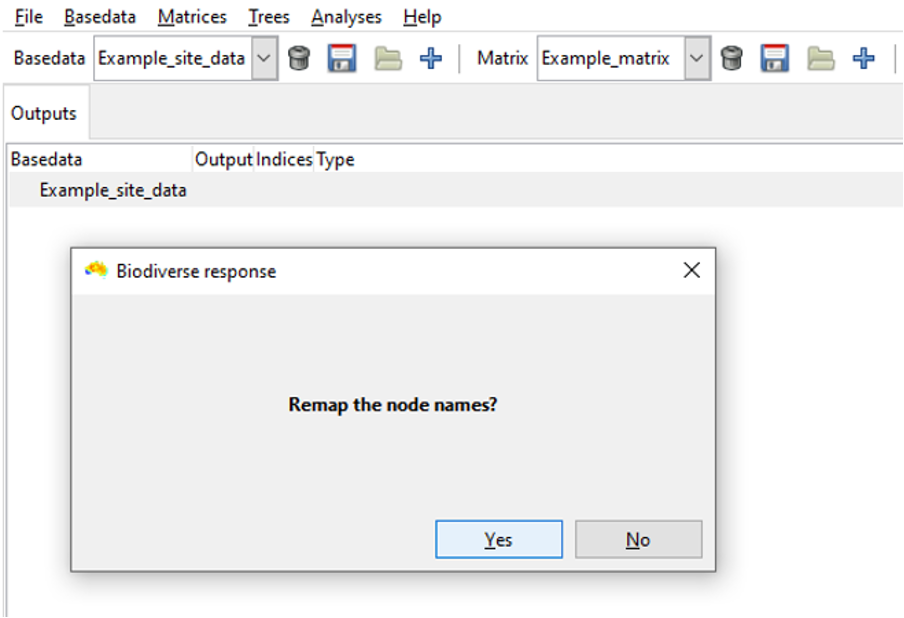
Since we are using the example input data, we will remap (but if you don’t wish to remap labels, simply click Cancel and the system will import the tree).
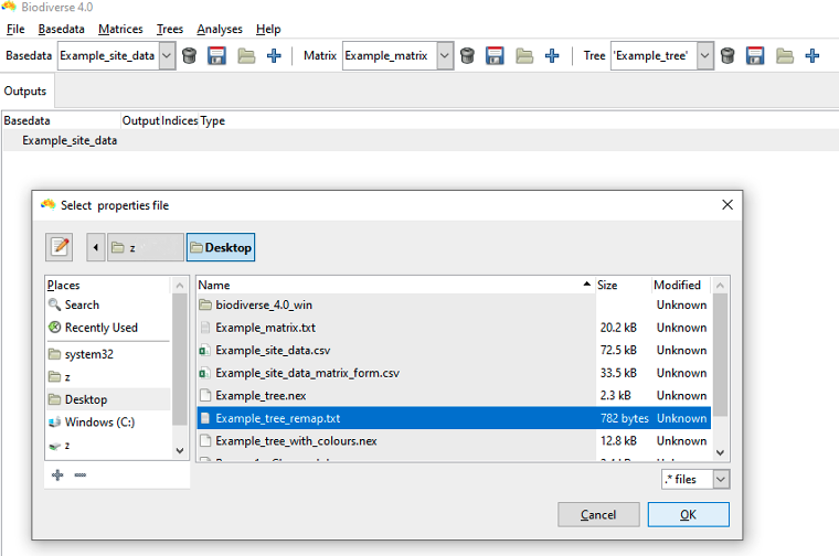
To remap the tree labels using an existing file, click YES. You are prompted to select a remap “label Source”. Here we use “user derived file” to select our Example_tree_remap.txt file. Click OK, accept the column separator and quote defaults, click Next.
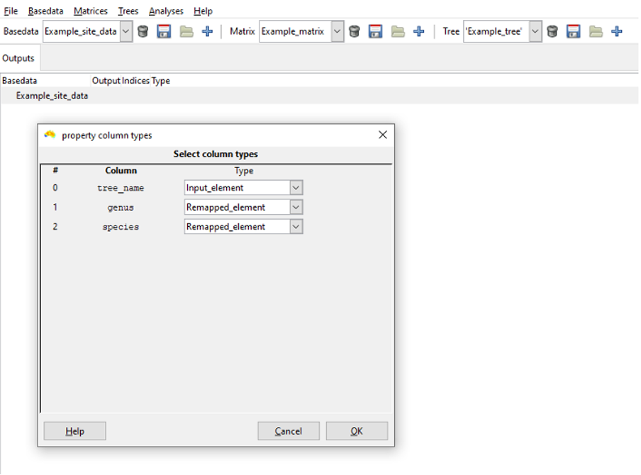
A popup dialog now prompts you to specify the column types for the remap process. Specify as many input_element columns as the tree labels have (i.e. one for nexus files) and then each label column in the BaseData object must be designated as a remapped_element. Click OK. The system will import the tree and perform the remapping.
Deriving a Tree You can derive a Tree from a BaseData object or Matrix at any time. Select the “Create tree from labels” or “Convert matrix to tree” options under the BaseData and Matrix menus, respectively:
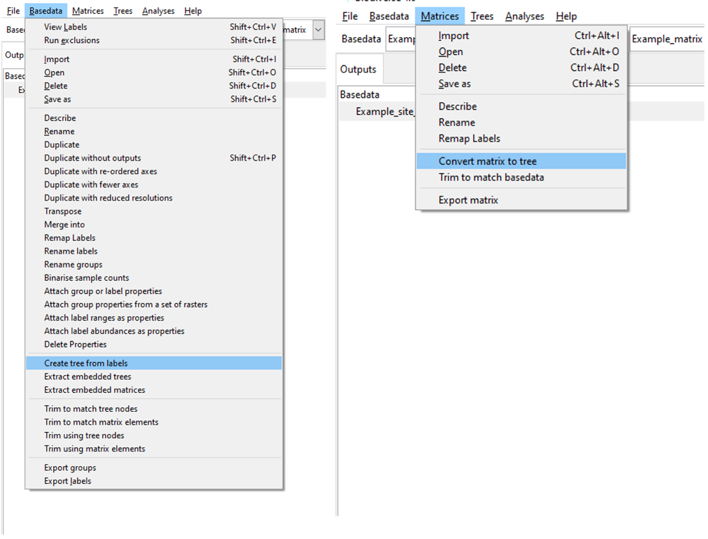
When generating a tree from the BaseData labels, labels are treated as taxonomic names, and thus are useful if the labels have at least two components (e.g. genus and species). A tree generated from a matrix is simply a cluster analysis using the average linkage function, so will only be valid for dissimilarity matrices.